Lab 10: Launching a PacBio assembly

Step 1: What is haplotype-aware assembly?

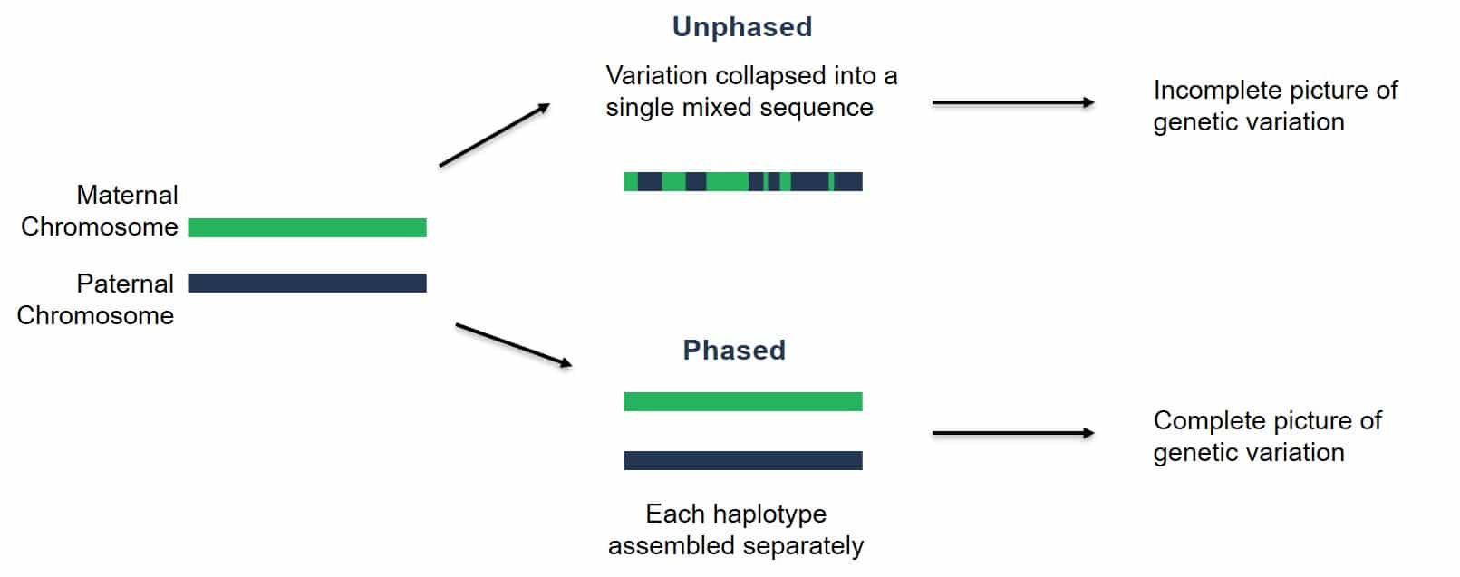
Diploid genomes contain two copies of every chromosome. We call each of these copies a haplotype. Our new goal for genome assembly is to produce a haplotype-resolved assembly. Take the example below: two chromosome haplotypes, one from the maternal contribution and the other from the paternal contribution. Over the last decade, many genome assemblies have been produced that smash the two haplotypes together, switching between maternal/paternal haplotypes in a single chromosome representation of the assembly. In other words, these chromosome assemblies are incomplete.

Nowadays, we have better data that is longer and more accurate. Given sufficient heterozygosity in a sample, we can phase the chromosome haplotypes. In other words, we can produce two genome assemblies for every diploid genome.

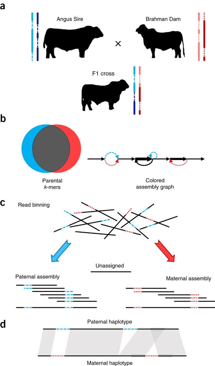
One issue is that without some additional information from the two parents of a diploid individual, we don’t often know which haplotype comes from the maternal versus paternal lineage. That is, unless you can also sequence the genomes of the parents! Here’s an example:

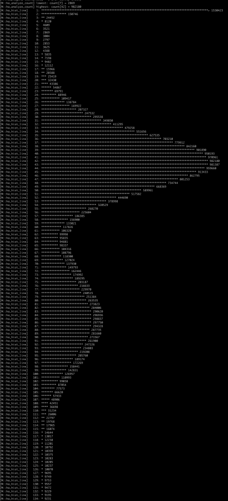
Okay, let’s review the basics of PacBio hifiasm assembler. Hifiasm leverages both the long PacBio reads, and k-mers derived from those reads, to identify 1) errors in the PacBio data, and 2) putative heterozygous allele sites in the data. First, it effectively recapitulates what you did with GenomeScope: it builds a k-mer distribution from the raw reads to identify a homozygous and heterozygous peak and their coverages.

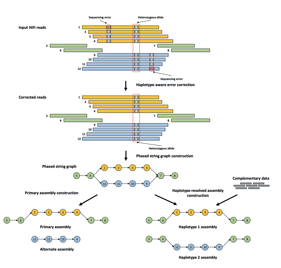
Credit: hifiasm (Heng Li)

Then, hifiasm builds an OLC graph that finds a path through heterozygous alleles — they look like bubbles in the graph. Hifiasm can produce two kinds of assemblies — primary + alt (left), or a phased haplotype 1 + haplotype 2 assembly. The “primary” assembly is the best path for one haplotype per contig. The “alt” is the alternative haplotype.

In this class, we generated two PacBio HiFi flow cells worth of data. Given our computational resources on the Virtual Machines (4 threads, 32 GB RAM) we can only use so much data as input. So I’ve subsetted the data to be smaller, so that it can still run on our VMs. I subsetted the data to 14 Gigabases (Gb) of the longest reads from a cell.

# data in /scratch/raw-data/PacBio
# pear.1M.subset.fastq.gz

Check out the hifiasm github page. Install the software on your own. Here’s the example on the github page for how to assemble heterozygous genomes:

# Assemble heterozygous genomes with built-in duplication purging
hifiasm -o HG002.asm -t32 HG002-file1.fq.gz HG002-file2.fq.gz

Before running hifiasm, read the tutorial first: https://hifiasm.readthedocs.io/en/latest/pa-assembly.html#pa-assembly

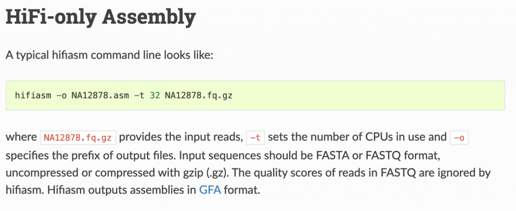
Remember that you only have 4 threads, so adjust -t accordingly. Launch your job using the pear.subset.1M.fastq.gz HiFi reads. You can use whatever prefix for -o that you would like.

After your assembly finishes:

1. The assembly file that we’ll focus on is the primary contig assembly. But it’s in a .gfa format….Find a solution on google to convert “pear.subset.gfa.bp.p_ctg.gfa” to a .fasta file.
2. Then use the assemblathon_stats.pl script to calculate basic statistics about your assembly. What is the total size, what is the contig N50?

Step 1: Understand the output

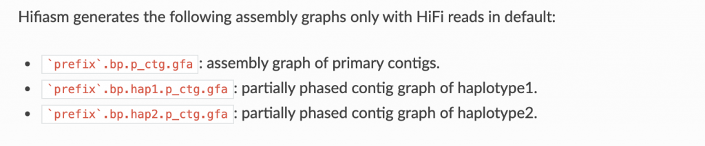
Hifiasm outputs a handful of files:

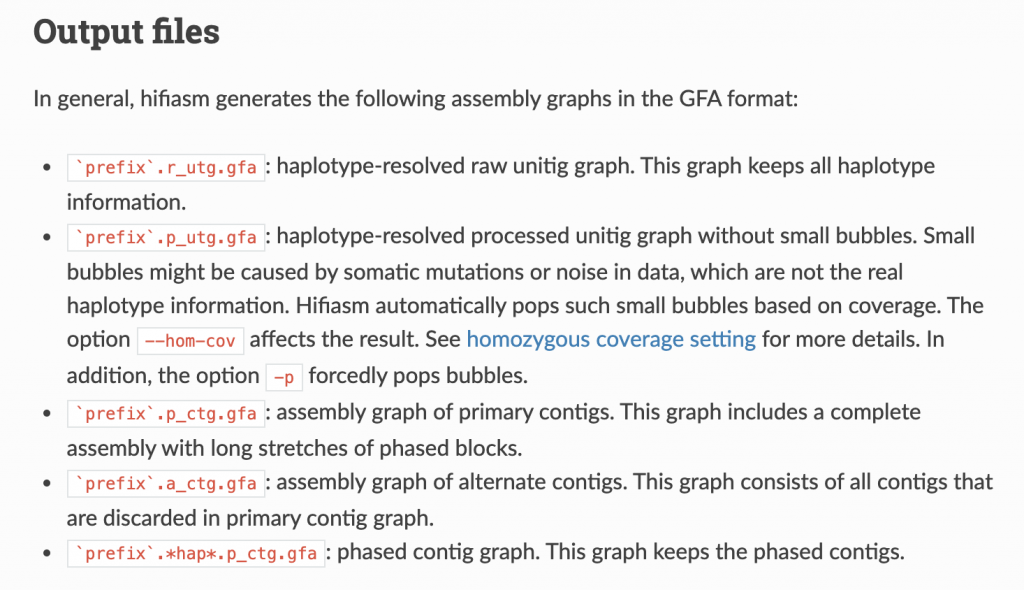
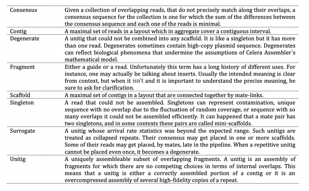
Let’s go over some of this terminology, first. The PacBio manual is quite helpful here:

For your assembly, using just the HiFi reads, you produced an assembly like on the left. Just the primary contigs :

Step 2: Get the basic stats.

You should have run assemblathon_stats.pl on your “pear.subset.gfa.bp.p_ctg.fasta” assembly. It reports a handful of statistics, both on the contigs and the scaffolds. We’ll talk about the difference between these two things in class. In short, scaffolds have gaps (NNNNNNNN) of unknown length that connect contigs together. Contigs are contiguous, meaning no gaps.

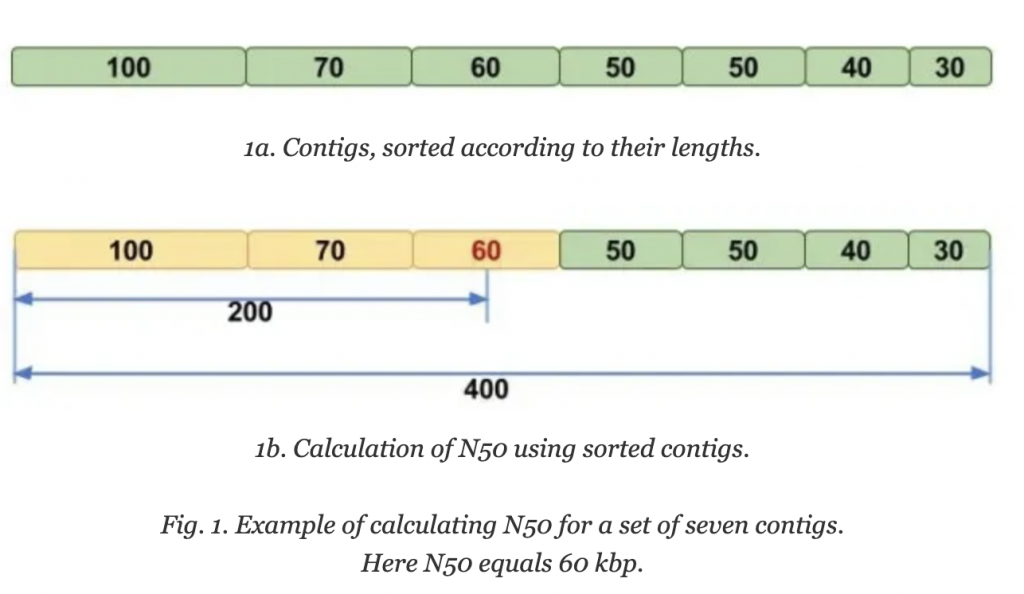
Molecular Ecologist describes N50 in a simple way: Imagine that you line up all the contigs in your assembly in the order of their sequence lengths (Fig. 1a). You have the longest contig first, then the second longest, and so on with the shortest ones in the end. Then you start adding up the lengths of all contigs from the beginning, so you take the longest contig + the second longest + the third longest and so on — all the way until you’ve reached the number that is making up 50% of your total assembly length. That length of the contig that you stopped counting at, this will be your N50 number.

 

Step 2: Figure out the lengths of contigs

Here’s another one of those one-liners that I keep around in my back pocket for things like this. Change “assembly.fasta” to whatever your assembly is called.

cat assembly.fasta |awk '$0 ~ ">" {if (NR > 1) {print c;} c=0;printf substr($0,2,100) "\t"; } $0 !~ ">" {c+=length($0);} END { print c; }' | awk '{print $1,$3}' | sort -nk 2

You can copy/paste this into Excel or Google Sheets if that helps. How many haploid chromosome does Q. virginiana have? How many large contigs do we have? Wow !

Step 3: Check out the assembly produced with ALL of the data, using the Hi-C integrated build

When you add in Hi-C data to the assembly process, hifiasm is allowed to use an additional data type to phase the two haplotypes. I’ve run the exact same command as you all, adding both flow cells worth of data, plus the Hi-C data, and started a hifiasm run. Just like the assembly on the right side:

The output that matters the most to us, the two phased haplotype fasta files, can be found in scratch:

hifiasm.hic.gfa.hic.hap1.p_ctg.fasta

hifiasm.hic.gfa.hic.hap2.p_ctg.fasta

First, we want to see how similar these two assemblies are in terms of length.

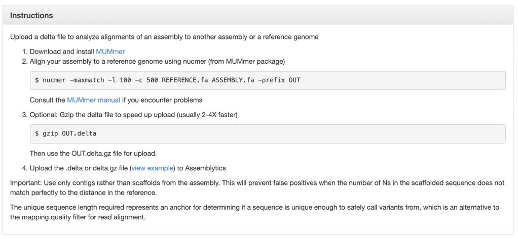
Next, how different are they in terms of structural variations? Assemblytics is a nifty online GUI that can build dotplots that compare two reference genome assemblies. Download and install MUMMER (https://sourceforge.net/projects/mummer/files/mummer/3.23/).

If you use Conda, make sure you download MUMMER3 and NOT MUMMER4, or else everything will break.

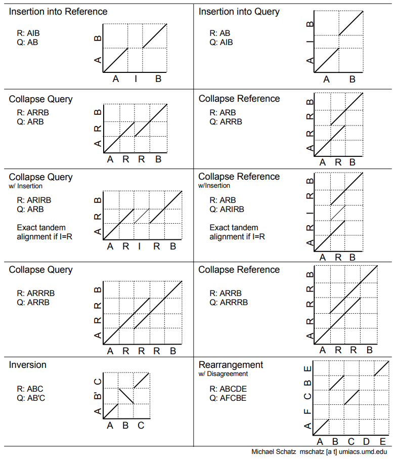
I keep this dotplot reference handy for how to interpret dotplots that compare a Reference versus a Query.

Step 1: Run Assemblytics

How similar are our two haplotypes? Which haplotype do we want to move forward with for scaffolding with Hi-C? Assemblytics is a nifty and quick way to quickly build dot plots that compare to sequences (or sets of sequences, e.g. in fasta files).

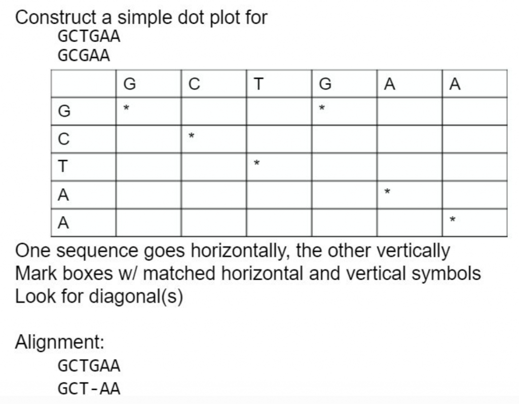
A dot plot is a graphical method that allows the comparison of two biological sequences and identify regions of close similarity between them. It is probably the oldest way of comparing two sequences [Maizel and Lenk, 1981].

Dot plot are two dimensional graphs, showing a comparison of two sequences. The principle used to generate the dot plot is: The top X and the left y axes of a rectangular array are used to represent the two sequences to be compared.

Calculation: Matrix
• Columns = residues of sequence 1
• Rows = residues of sequence 2.
A dot is plotted at every co-ordinate where there is similarity between the bases.

What about an example with longer sequences? Plus repeats!

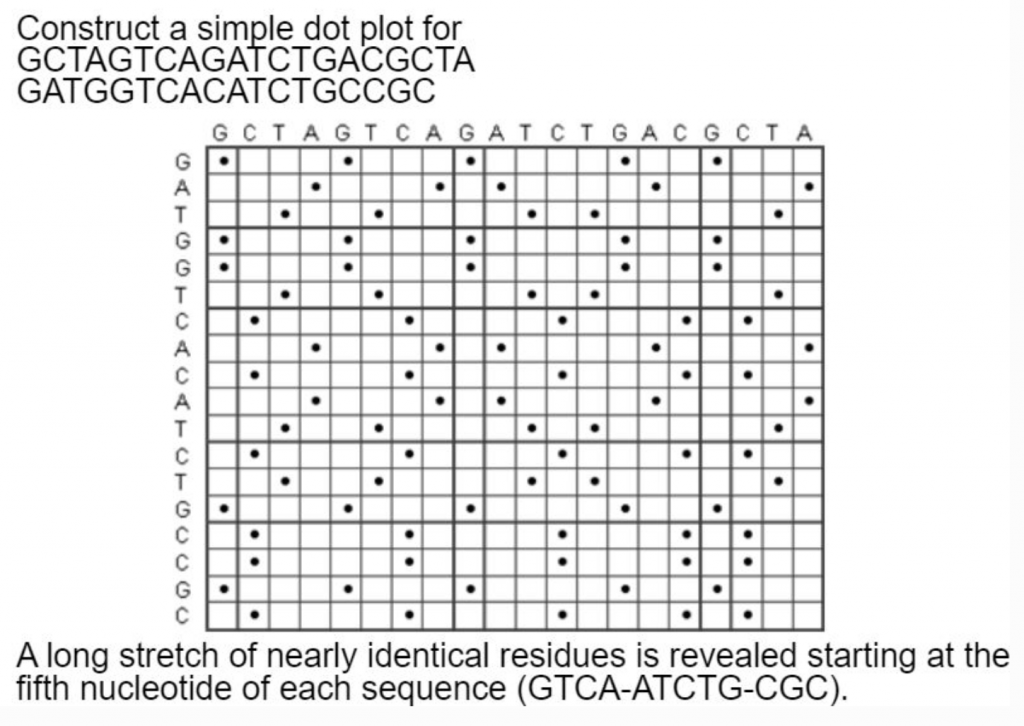
Simple dot plots get too noisy when comparing every single nucleotide in a string. The solution is to compare windows of strings.

Install MUMMER and run assemblytics, just as the online instructions tell you to.

Depending on how you installed it, you might run into some problems.

Setting the window size of matches

We use the -l 100 and -c 500 options for Assemblytics, per the online manual. Check out the nucmer manual for what these options mean:

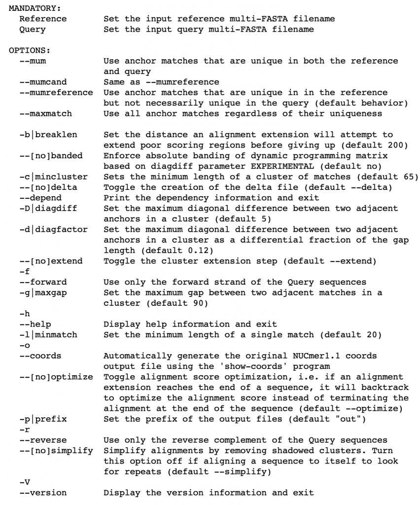
-l 100 means that a minimum match between two sequence strings must be at least 100 nucleotides. -c 500 means that we must have several overlapping matches that equal at least 500 nucleotides. Only alignments matching these two parameters will be output. This filters out quite a bit of noise, especially in our case, since the two haplotypes should be *fairly* similar (~1.5% heterozygous).